Technical notes on using a virtual WPS/WRF environment
Overview
The WRF distribution created through the process outlined in WPS/WRF Install provides a static collection of a fully-compiled and installed WPS and WRF environment (at a later date, it may contain more). Through its use (typically through copying and/or linking) we may be confident that we are using a fully-tested, operational environment for a wide variety of applications. Users or developers who want different distributions can simply install them in a similar manner, storing them in different locations. With this approach, we can have a collection of stable distributions of different versions, and experimental distributions.
Within the WRF distribution is the custom wrfusersetup.py program, which is used to create a new WRF environment in a user directory. This environment consists of a directory named by the user, with a large number of links, and in some cases, copies, to files in the static distribution. This local environment may then be modified and used for custom WPS/WRF activities without affecting the primary distribution. In this way, a user can create one or more separate WRF environments for independent simulations.
Use of the wrfusersetup.py program is relatively simple - the user invokes it with a single argument of the name of the directory (and an optional path to it) that should be used for the simulation. The directory name provided must be writable by the user, of course, and if it already exists then it will not proceed. This policy is implemented to ensure that users don’t accidentally overwrite a simulation directory that might have a lot of important data in it.
The following demonstration goes through the process of creating a single virtual WPS/WRF environment and running all of the preprocessing and simulation stages within it. This is the way a typical WRF user would interact with the model components. Although not important to understand at this point, EHRATM processes will create a single virtual WPS/WRF environment for each preprocessing and simulation stage. The reason for this is to support flexibility in a structure of loosely-coupled components. In this way, users are able to create custom workflows and not be restricted as one might in a single virtual environment. Additionally, users who need to do do some low-level debugging or experimentation can do so in a very restricted environment without the complexities of a full model run.
Creation of a WPS/WRF run environment for custom simulation
In these examples, I’m assuming a WPS/WRF distribution has been created (using guidance provided in WPS/WRF Install) in /dvlscratch/ATM/morton/WRFDistributions/WRFV4.3/ and that I’m starting with /dvlscratch/ATM/morton/ as my cwd. First, I run wrfusersetup.py with no argument, getting the usage message, then I run it with the MyFirstTest argument, indicating that I want a local WPS/WRF distribution to be created in that directory:
$ pwd
/dvlscratch/ATM/morton

$ WRFDistributions/WRFV4.3/wrfusersetup.py


Usage: ./wrfusersetup.py <DomainName>

                 or

        /path/to/wrfusersetup.py /path/to/<DomainName>

     * Creates dir <DomainName> in specified directory


$ WRFDistributions/WRFV4.3/wrfusersetup.py MyFirstTest
WRF src distribution directory: /dvlscratch/ATM/morton/WRFDistributions/WRFV4.3
geog data dir: /dvlscratch/ATM/morton/WRFDistributions/WRFV4.3/GEOG_DATA
Creating domain: MyFirstTest in directory: /dvlscratch/ATM/morton
Setting up WPS run dir: /dvlscratch/ATM/morton/MyFirstTest/WPS
Done creating geogrid items
Done creating metgrid items
Done creating ungrib items
Done creating util items
Setting up WRF run dir: /dvlscratch/ATM/morton/MyFirstTest/WRF
WRF run dir set up completed
Once complete, I can take a quick look in this new directory:
$ tree -L 1 MyFirstTest
MyFirstTest
├── GEOG_DATA -> /dvlscratch/ATM/morton/WRFDistributions/WRFV4.3/GEOG_DATA
├── WPS
└── WRF

3 directories, 0 files

$ tree -L 1 MyFirstTest/WPS
MyFirstTest/WPS
├── geogrid
├── geogrid.exe -> /dvlscratch/ATM/morton/WRFDistributions/WRFV4.3/WPS/geogrid/src/geogrid.exe
├── link_grib.csh
├── metgrid
├── metgrid.exe -> /dvlscratch/ATM/morton/WRFDistributions/WRFV4.3/WPS/metgrid/src/metgrid.exe
├── namelist.wps
.
.
.
├── ungrib.exe -> /dvlscratch/ATM/morton/WRFDistributions/WRFV4.3/WPS/ungrib/src/ungrib.exe
└── util

4 directories, 10 files


$ tree -L 1 MyFirstTest/WRF
MyFirstTest/WRF
├── aerosol.formatted -> /dvlscratch/ATM/morton/WRFDistributions/WRFV4.3/WRF/run/aerosol.formatted
├── aerosol_lat.formatted -> /dvlscratch/ATM/morton/WRFDistributions/WRFV4.3/WRF/run/aerosol_lat.formatted
.
.
.
├── MPTABLE.TBL -> /dvlscratch/ATM/morton/WRFDistributions/WRFV4.3/WRF/run/MPTABLE.TBL
├── namelist.input
├── ndown.exe -> /dvlscratch/ATM/morton/WRFDistributions/WRFV4.3/WRF/main/ndown.exe
├── ozone.formatted -> /dvlscratch/ATM/morton/WRFDistributions/WRFV4.3/WRF/run/ozone.formatted
.
.
.
├── wind-turbine-1.tbl -> /dvlscratch/ATM/morton/WRFDistributions/WRFV4.3/WRF/run/wind-turbine-1.tbl
└── wrf.exe -> /dvlscratch/ATM/morton/WRFDistributions/WRFV4.3/WRF/main/wrf.exe

0 directories, 81 files
The WPS and WRF directories are fully functional, ready for use to set up and run a simulation. Note that namelist.wps and namelist.input are copies of files, not linked to the original execution. In the following, I demonstrate how this new run directory can be used to manually set up and execute a simple WRF simulation using GFS files from CTBTO’s filesystem. My assumption is that the reader is experienced in running WRF simulations, so I don’t bother to explain the steps in any detail.
Demonstration of the newly-created WPS/WRF run environment
For this example, we will arbitrarily choose to run a simple model over the Anchorage region of Alaska for 18 hours, using met data from CTBTO’s GFS archive, running from 00Z to 18Z on 21 February 2021. The steps we’ll take
Create a domain by editing namelist.wps, run geogrid.exe, and verify a reasonable-looking domain with ncview
Ungrib the metfiles
Run metgrid and, again, do a quick, random check of the output files with ncview
Run real, and a quick view of the output files
Run wrf, and a quick view of the output files
All of this is performed on dls011 in /dvlscratch/ATM/morton/MyFirstTest/
$ cd WPS
and edit namelist.wps for the domain and times of interest
&share
 wrf_core = 'ARW',
 max_dom = 1,
 start_date = '2021-02-21_00:00:00','2019-09-04_12:00:00',
 end_date   = '2021-02-21_18:00:00','2019-09-04_12:00:00',
 interval_seconds = 10800
/

&geogrid
 parent_id         =   1,   1,
 parent_grid_ratio =   1,   3,
 i_parent_start    =   1,  53,
 j_parent_start    =   1,  25,
 e_we              =  70, 220,
 e_sn              =  60, 214,
 geog_data_res = 'default','default',
 dx = 15000,
 dy = 15000,
 map_proj = 'lambert',
 ref_lat   =  61.22,
 ref_lon   = -149.90,
 truelat1  =  30.0,
 truelat2  =  60.0,
 stand_lon = -149.90,
 geog_data_path = '../GEOG_DATA'
/

&ungrib
 out_format = 'WPS',
 prefix = 'FILE',
/

&metgrid
 fg_name = 'FILE'
/
Run geogrid
$ ./geogrid.exe
Parsed 49 entries in GEOGRID.TBL
Processing domain 1 of 1
  Processing XLAT and XLONG
  Processing MAPFAC
.
.
.
!!!!!!!!!!!!!!!!!!!!!!!!!!!!!!!!!!!!!!!!!!!!!
!  Successful completion of geogrid.        !
!!!!!!!!!!!!!!!!!!!!!!!!!!!!!!!!!!!!!!!!!!!!!
and then use ncview to sample a couple of fields from the newly-created geo_em.d01.nc. Note that I have placed a copy of the ncview binary in the repo, in component_dev/python3/test/ncview so for convenience I assign the path to an environment variable
$ export NCVIEW=/dvlscratch/ATM/morton/git/hratm-experimentation/component_dev/python3/test/ncview

$ $NCVIEW geo_em.d01.nc
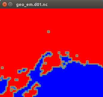
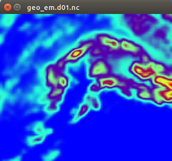
LANDMASK on the left, HGT_M (terrain height) on the right
Then, we set up and run ungrib, using the following GFS met files
$ ls -l /ops/data/atm/live/ncep/2021/02/21/0.5.fv3
total 0
-rw-r--r--. 1 auto auto 90149857 Feb 21  2021 GD21022100
-rw-r--r--. 1 auto auto 98203239 Feb 21  2021 GD21022103
-rw-r--r--. 1 auto auto 90765897 Feb 21  2021 GD21022106
-rw-r--r--. 1 auto auto 98680596 Feb 21  2021 GD21022109
-rw-r--r--. 1 auto auto 90952126 Feb 21  2021 GD21022112
-rw-r--r--. 1 auto auto 99666513 Feb 21  2021 GD21022115
-rw-r--r--. 1 auto auto 91186765 Feb 21  2021 GD21022118
-rw-r--r--. 1 auto auto 99238842 Feb 21  2021 GD21022121
Remaining in the WPS/ directory, we make the links to the met files and Vtable
$ ./link_grib.csh /ops/data/atm/live/ncep/2021/02/21/0.5.fv3/GD*

$ ls -l GRIBFILE*
lrwxrwxrwx. 1 morton consult 53 Sep 21 01:24 GRIBFILE.AAA -> /ops/data/atm/live/ncep/2021/02/21/0.5.fv3/GD21022100
lrwxrwxrwx. 1 morton consult 53 Sep 21 01:24 GRIBFILE.AAB -> /ops/data/atm/live/ncep/2021/02/21/0.5.fv3/GD21022103
lrwxrwxrwx. 1 morton consult 53 Sep 21 01:24 GRIBFILE.AAC -> /ops/data/atm/live/ncep/2021/02/21/0.5.fv3/GD21022106
lrwxrwxrwx. 1 morton consult 53 Sep 21 01:24 GRIBFILE.AAD -> /ops/data/atm/live/ncep/2021/02/21/0.5.fv3/GD21022109
lrwxrwxrwx. 1 morton consult 53 Sep 21 01:24 GRIBFILE.AAE -> /ops/data/atm/live/ncep/2021/02/21/0.5.fv3/GD21022112
lrwxrwxrwx. 1 morton consult 53 Sep 21 01:24 GRIBFILE.AAF -> /ops/data/atm/live/ncep/2021/02/21/0.5.fv3/GD21022115
lrwxrwxrwx. 1 morton consult 53 Sep 21 01:24 GRIBFILE.AAG -> /ops/data/atm/live/ncep/2021/02/21/0.5.fv3/GD21022118
lrwxrwxrwx. 1 morton consult 53 Sep 21 01:24 GRIBFILE.AAH -> /ops/data/atm/live/ncep/2021/02/21/0.5.fv3/GD21022121

$ ln -sf ungrib/Variable_Tables/Vtable.GFS Vtable

$ ls -l Vtable
lrwxrwxrwx. 1 morton consult 33 Sep 21 01:25 Vtable -> ungrib/Variable_Tables/Vtable.GFS
And then go ahead and run and verify that expected output files are present
$ ./ungrib.exe
.
.
.
!!!!!!!!!!!!!!!!!!!!!!!!!!!!!!!!!!!!!!!
!  Successful completion of ungrib.   !
!!!!!!!!!!!!!!!!!!!!!!!!!!!!!!!!!!!!!!!


$ ls -l FILE*
-rw-r--r--. 1 morton consult 204862664 Sep 21 01:26 FILE:2021-02-21_00
-rw-r--r--. 1 morton consult 204862664 Sep 21 01:27 FILE:2021-02-21_03
-rw-r--r--. 1 morton consult 204862664 Sep 21 01:27 FILE:2021-02-21_06
-rw-r--r--. 1 morton consult 204862664 Sep 21 01:27 FILE:2021-02-21_09
-rw-r--r--. 1 morton consult 204862664 Sep 21 01:27 FILE:2021-02-21_12
-rw-r--r--. 1 morton consult 204862664 Sep 21 01:27 FILE:2021-02-21_15
-rw-r--r--. 1 morton consult 204862664 Sep 21 01:27 FILE:2021-02-21_18
Finally, to wrap up the WPS preprocessing, we run metgrid, then do a quick spot-verification of the output.
$ export MPIRUN=/usr/lib64/openmpi/bin/mpirun

$ $MPIRUN -np 4 ./metgrid.exe
Processing domain 1 of 1
 Processing 2021-02-21_00
    FILE
 Processing 2021-02-21_03
    FILE
Processing 2021-02-21_06
    FILE
 Processing 2021-02-21_09
    FILE
 Processing 2021-02-21_12
    FILE
 Processing 2021-02-21_15
    FILE
 Processing 2021-02-21_18
    FILE
!!!!!!!!!!!!!!!!!!!!!!!!!!!!!!!!!!!!!!!
!  Successful completion of metgrid.  !
!!!!!!!!!!!!!!!!!!!!!!!!!!!!!!!!!!!!!!!

$ ls -l met_em*
-rw-r--r--. 1 morton consult 8451668 Sep 21 01:30 met_em.d01.2021-02-21_00:00:00.nc
-rw-r--r--. 1 morton consult 8451668 Sep 21 01:31 met_em.d01.2021-02-21_03:00:00.nc
-rw-r--r--. 1 morton consult 8451668 Sep 21 01:31 met_em.d01.2021-02-21_06:00:00.nc
-rw-r--r--. 1 morton consult 8451668 Sep 21 01:31 met_em.d01.2021-02-21_09:00:00.nc
-rw-r--r--. 1 morton consult 8451668 Sep 21 01:31 met_em.d01.2021-02-21_12:00:00.nc
-rw-r--r--. 1 morton consult 8451668 Sep 21 01:31 met_em.d01.2021-02-21_15:00:00.nc
-rw-r--r--. 1 morton consult 8451668 Sep 21 01:31 met_em.d01.2021-02-21_18:00:00.nc


$ $NCVIEW met_em.d01.2021-02-21_12:00:00.nc

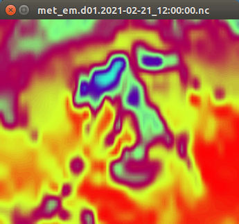
HGT_M (terrain height) on the left, 5th vertical level RH on right
This concludes the WPS preprocessing, so we next to into the WRF directory
$ cd ../WRF
edit namelist.input (I’m just showing the first two sections of it here)
&time_control
 run_days                            = 0,
 run_hours                           = 18,
 run_minutes                         = 0,
 run_seconds                         = 0,
 start_year                          = 2021, 2019,
 start_month                         = 02,   09,
 start_day                           = 21,   04,
 start_hour                          = 00,   12,
 end_year                            = 2021, 2019,
 end_month                           = 02,   09,
 end_day                             = 21,   06,
 end_hour                            = 18,   00,
 interval_seconds                    = 10800
 input_from_file                     = .true.,.true.,
 history_interval                    = 60,  60,
 frames_per_outfile                  = 1, 1,
 restart                             = .false.,
 restart_interval                    = 7200,
 io_form_history                     = 2
 io_form_restart                     = 2
 io_form_input                       = 2
 io_form_boundary                    = 2
 /

 &domains
 time_step                           = 45,
 time_step_fract_num                 = 0,
 time_step_fract_den                 = 1,
 max_dom                             = 1,
 e_we                                = 70,    220,
 e_sn                                = 60,    214,
 e_vert                              = 45,     45,
 dzstretch_s                         = 1.1
 p_top_requested                     = 5000,
 num_metgrid_levels                  = 34,
 num_metgrid_soil_levels             = 4,
 dx                                  = 15000,
 dy                                  = 15000,
 grid_id                             = 1,     2,
 parent_id                           = 0,     1,
 i_parent_start                      = 1,     53,
 j_parent_start                      = 1,     25,
 parent_grid_ratio                   = 1,     3,
 parent_time_step_ratio              = 1,     3,
 feedback                            = 1,
 smooth_option                       = 0
 /
 .
 .
 .
make the links to the met_em files in ../WPS/ and run real
$ ln -sf ../WPS/met_em* .
$ ls -l met_em*
lrwxrwxrwx. 1 morton consult 40 Sep 21 01:40 met_em.d01.2021-02-21_00:00:00.nc -> ../WPS/met_em.d01.2021-02-21_00:00:00.nc
lrwxrwxrwx. 1 morton consult 40 Sep 21 01:40 met_em.d01.2021-02-21_03:00:00.nc -> ../WPS/met_em.d01.2021-02-21_03:00:00.nc
.
.
.
lrwxrwxrwx. 1 morton consult 40 Sep 21 01:40 met_em.d01.2021-02-21_18:00:00.nc -> ../WPS/met_em.d01.2021-02-21_18:00:00.nc


$ $MPIRUN -np 4 ./real.exe
 starting wrf task            0  of            4
 starting wrf task            1  of            4
 starting wrf task            2  of            4
 starting wrf task            3  of            4
this runs quickly, and the ongoing status can be viewed in rsl.error.0000
$ tail rsl.error.0000
d01 2021-02-21_18:00:00 Turning off use of TROPOPAUSE level data in vertical interpolation
Using sfcprs3 to compute psfc
d01 2021-02-21_18:00:00 No average surface temperature for use with inland lakes
 Assume Noah LSM input
d01 2021-02-21_18:00:00 forcing artificial silty clay loam at   15 points, out of   1050
d01 2021-02-21_18:00:00 Total post number of sea ice location changes (water to land) =     14
d01 2021-02-21_18:00:00 Timing for processing          0 s.
d01 2021-02-21_18:00:00 Timing for output          0 s.
d01 2021-02-21_18:00:00 Timing for loop #    7 =          0 s.
d01 2021-02-21_18:00:00 real_em: SUCCESS COMPLETE REAL_EM INIT
Then, we verify that output files are present and spot-check with ncview
$ ls -l wrf[bi]*
-rw-r--r--. 1 morton consult 35525008 Sep 21 01:43 wrfbdy_d01
-rw-r--r--. 1 morton consult 18493628 Sep 21 01:43 wrfinput_d01

$ $NCVIEW wrfinput_d01
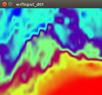
T2 field from wrfinput initial conditions
Finally, we run the simulation! Everything should be in place, so we just run it
$ $MPIRUN -np 4 ./wrf.exe
starting wrf task            0  of            4
starting wrf task            1  of            4
starting wrf task            2  of            4
starting wrf task            3  of            4
This took about 14 minutes on dls011 (where these four tasks were the only significant load on the system), so ongoing progress can be monitored as follows
$ tail -f rsl.error.0000
.
.
.
Timing for main: time 2021-02-21_17:58:30 on domain   1:    0.31064 elapsed seconds
Timing for main: time 2021-02-21_17:59:15 on domain   1:    0.31115 elapsed seconds
Timing for main: time 2021-02-21_18:00:00 on domain   1:    0.31203 elapsed seconds
 mediation_integrate.G        1944 DATASET=HISTORY
 mediation_integrate.G        1945  grid%id            1  grid%oid            2
Timing for Writing wrfout_d01_2021-02-21_18:00:00 for domain        1:    0.28613 elapsed seconds
d01 2021-02-21_18:00:00 wrf: SUCCESS COMPLETE WRF
When complete, we verify the expected wrfout files are present, and spot-check with ncview
$ ls -l wrfout*
-rw-r--r--. 1 morton consult 19332628 Sep 21 01:52 wrfout_d01_2021-02-21_00:00:00
-rw-r--r--. 1 morton consult 19332628 Sep 21 01:52 wrfout_d01_2021-02-21_01:00:00
.
.
.
-rw-r--r--. 1 morton consult 19332628 Sep 21 02:00 wrfout_d01_2021-02-21_17:00:00
-rw-r--r--. 1 morton consult 19332628 Sep 21 02:01 wrfout_d01_2021-02-21_18:00:00


$ $NCVIEW wrfout_d01_2021-02-21_18:00:00
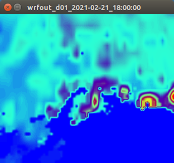
SNOW field from the last wrfout file
And, that’s it! MISSION ACCOMPLISHED
Summary
For someone used to running WPS and WRF, this was probably boring, but for the less experienced user, hopefully it serves as a little bit of guidance, and demonstrates how we can quickly create and execute a custom WRF simulation driven by CTBTO GFS data.
After the demo described above, we could create more local run directories for a variety of simulations. Perhaps we just want to try the same simulation with different physics parameterisations. One approach would be to create different run directories for each case and, in each, go through the above steps with slightly different versions of namelist.input, each using different parameters.